Cohort Analysis: Using RFM and Clustering

24/8/2020 9-minute read

What is RFM Model

RFM model is one of the customer valuation model. RFM is shorthand of Recency, Frequency and Money. This model classifies customers through the three cateogries, and different operation strategies can be adopted for different types of users, or use classifiers such as logistic regression, decision trees, etc. to predict the future behavior of users, and do some recommendation strategies.

The definitions of the three metrics are:

Recency: The time interval between now and last purchase
Frequency: The total number of actions of a user
Monetary Value: The total consumption amount of a user

Generally speaking, since the three indicators are continuous, it is necessary to divide each indicator into different intervals according to the size of the number . Specifically, how to divide and determine the boundaries of division can be combined with the needs of the business. For example:

An online ordering platform dismantled the three metrics into more detailed metrics:

T(Time) is divided as: recent 3 months (t1), in the past 3-12 months (t2), 12 months ago (t3)
R: the interval between now and last expected action date (R1), the interval between now and last active date (R2)
F: number of orders of a user (F1), active days of a user (F2), number of Page Views of a user (F3)

M: Total money ordered
Then we naturally have:
$$R = r_1 * R_1 + r_2 * R_2 $$
$$F = t_1 * (f_1 * F_1 + f_2 * F_2 + f_3 * F_3)+t_2(…)+t_3(…)$$
Where the small cases represent weights for each metrics. So according to the above calculation, we can calculate R, F, M value for each user and classify them as:

Category	#Users	Description	Tag
1		Almost gone
2		Not active (Judging by T)
3		Relatively low (e.g., has a order 3 months ago)
4		R low, F & M high (e.g., was high value)
5		F low M high
6		F high M low
7		R, F, M high

Not every category worths notice, and F varied case by case. A general classification would be growth metrics and profit related metrics, and deviding into smaller granuality accordingly.

Now let’s build a RFM model using R, first we do it by rules then we use clustering.

Data Description

Let’s use the Online Retail Dataset provided by UCI Machine Learning Repository, it contains about 50w transaction data of a UK outlet from 01/12/2010 to 09/12/2011.

    > str(trx)
    tibble [541,909 x 8] (S3: tbl_df/tbl/data.frame)
     $ InvoiceNo  : chr [1:541909] "536365" "536365" "536365" "536365" 
     $ StockCode  : chr [1:541909] "85123A" "71053" "84406B" "84029G" 
     $ Description: chr [1:541909] "WHITE HANGING HEART T-LIGHT HOLDER" "WHITE METAL LANTERN" "CREAM CUPID HEARTS COAT HANGER" "KNITTED UNION FLAG HOT WATER BOTTLE"
     $ Quantity   : num [1:541909] 6 6 8 6 6 2 6 6 6 32 
     $ InvoiceDate: POSIXct[1:541909], format: "2010-12-01 08:26:00" "2010-12-01 08:26:00" 
     $ UnitPrice  : num [1:541909] 2.55 3.39 2.75 3.39 3.39 7.65 4.25 1.85 1.85 1.69 
     $ CustomerID : num [1:541909] 17850 17850 17850 17850 17850 
     $ Country    : chr [1:541909] "United Kingdom" "United Kingdom" "United Kingdom" "United Kingdom"

Data Cleaning & Preparation

Drop NA and negative UnitPrice and Quantity:

trx <- trx %>% 
      mutate(Quantity = replace(Quantity, Quantity<=0, NA),
             UnitPrie = replace(UnitPrice, UnitPrice<=0, NA))
trx <- trx %>% na.omit(trx)

Change data type and calculate GMV per user:

trx <- trx %>% 
 mutate(InvoiceNo=as.factor(InvoiceNo), StockCode=as.factor(StockCode), 
 InvoiceDate=as.Date(InvoiceDate, ‘%m/%d/%Y’), CustomerID=as.factor(CustomerID), 
 Country=as.factor(Country))
trx <- trx %>%
mutate(GMV = Quantity*UnitPrice)
df_customer <- trx%>% select(CustomerID,InvoiceDate,GMV)

Now we calculate Recency, Frequency and Monetary. Recency is the time interval between now and last purchase; Frequency is non repetitive purchase; Monetary is the money spent:

analysis_date <- lubridate::as_date(‘2012–01–01’, tz = ‘UTC’)
df_RFM <- trx %>% 
group_by(CustomerID) %>% 
summarise(recency=as.numeric(analysis_date-max(InvoiceDate)),
frequency =n_distinct(InvoiceNo), monetary= sum(GMV))

Classification by Rules

We first classifies R, F, M by quantiles:

> summary(df_RFM)
   CustomerID      recency        frequency          monetary        
 12346  :   1   Min.   : 23.0   Min.   :  1.000   Min.   :     3.75  
 12347  :   1   1st Qu.: 40.0   1st Qu.:  1.000   1st Qu.:   307.42  
 12348  :   1   Median : 73.0   Median :  2.000   Median :   674.48  
 12349  :   1   Mean   :115.1   Mean   :  4.272   Mean   :  2054.27  
 12350  :   1   3rd Qu.:164.8   3rd Qu.:  5.000   3rd Qu.:  1661.74  
 12352  :   1   Max.   :396.0   Max.   :209.000   Max.   :280206.02  
 (Other):4332    

# assign scores to r,f,m based on quantiles
df_RFM$R_Score[df_RFM$recency>164.8]<-1
df_RFM$R_Score[df_RFM$recency>73 & df_RFM$recency<=164.8 ]<-2
df_RFM$R_Score[df_RFM$recency>40 & df_RFM$recency<=73 ]<-3
df_RFM$R_Score[df_RFM$recency<=40]<-4
#F_score
df_RFM$F_Score[df_RFM$frequency<1]<-1
df_RFM$F_Score[df_RFM$frequency>=1 & df_RFM$frequency<2]<-2
df_RFM$F_Score[df_RFM$frequency>=2 & df_RFM$frequency<5 ]<-3
df_RFM$F_Score[df_RFM$frequency>=5]<-4
#M_score
df_RFM$M_Score[df_RFM$monetary<= 307.42]<-1
df_RFM$M_Score[df_RFM$monetary>=307.42 & df_RFM$monetary<674.49]<-2
df_RFM$M_Score[df_RFM$monetary>=674.49 & df_RFM$monetary<1661.74 ]<-3
df_RFM$M_Score[df_RFM$monetary>=1661.74]<-4
#RFM_score
df_RFM<- df_RFM %>% mutate(RFM_Score = 100*R_Score + 10*F_Score+M_Score)

Then classifies users by the quantiles:

# Segments using RFM scores:
df_RFM$segmentRFM<-NULL
champions <- c(444)
loyal_customers <- c(334, 342, 343, 344, 433, 434, 443)
potential_loyalist <- c(332,333,341,412,413,414,431,432,441,442,421,422,423,424)
recent_customers <- c(411)
promising <- c(311, 312, 313, 331)
needing_attention <- c(212,213,214,231,232,233,241,314,321,322,323,324)
about_to_sleep <- c(211)
at_risk <- c(112,113,114,131,132,133,142,124,123,122,121,224,223,222,221)
cant_lose <- c(134,143,144,234,242,243,244)
hibernating <- c(141)
lost <- c(111)

df_RFM$segmentRFM[which(df_RFM$RFM_Score %in% champions)] = "Champions"
df_RFM$segmentRFM[which(df_RFM$RFM_Score %in% loyal_customers)] = "Loyal Customers"
df_RFM$segmentRFM[which(df_RFM$RFM_Score %in% potential_loyalist)] = "Potential Loyalist"
df_RFM$segmentRFM[which(df_RFM$RFM_Score %in% recent_customers)] = "Recent customers"
df_RFM$segmentRFM[which(df_RFM$RFM_Score %in% promising)] = "Promising"
df_RFM$segmentRFM[which(df_RFM$RFM_Score %in% needing_attention)] = "Customer Needing Attention"
df_RFM$segmentRFM[which(df_RFM$RFM_Score %in% about_to_sleep)] = "About to Sleep"
df_RFM$segmentRFM[which(df_RFM$RFM_Score %in% at_risk)] = "At Risk"
df_RFM$segmentRFM[which(df_RFM$RFM_Score %in% cant_lose)] = "Can’t Lose Them"
df_RFM$segmentRFM[which(df_RFM$RFM_Score %in% hibernating)] = "Hibernating"
df_RFM$segmentRFM[which(df_RFM$RFM_Score %in% lost)] = "Lost"

See what we got:

df_RFM %>%
  count(segmentRFM) %>%
  arrange(desc(n)) %>%
  rename(segmentRFM = segmentRFM, Count = n)
# A tibble: 8 x 2
  segmentRFM                 Count
  <chr>                      <int>
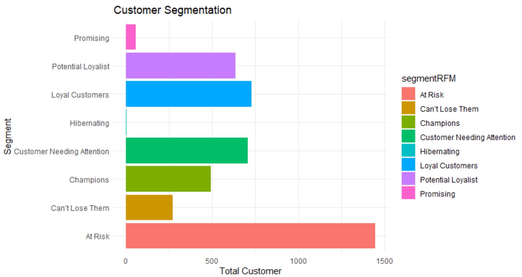
1 At Risk                     1448
2 Loyal Customers              728
3 Customer Needing Attention   706
4 Potential Loyalist           635
5 Champions                    494
6 Can’t Lose Them              270
7 Promising                     56
8 Hibernating                    1

and visualize:

#Visualization
library(ggplot2)
p1 <- ggplot(data = df_RFM) +
  aes(x = segmentRFM, fill = segmentRFM) +
  geom_bar() +
  labs(title = "Customer Segmentation",
       x = "Segment",
       y = "Total Customer") +coord_flip()+
  theme_minimal()
p1

We can adopt different strategies on different kinds of users:

For Champions, r, f, and m indicators are all very high, they may be loyal users of our brand, the first users of new products, and may help us spread the product, so these users need to be rewarded
For Loyal Customers, one or two of r, f, m are not very high. They can be recommended high-value products, and they can be invited to write about product experiences to keep them active.
For Potential Loyalist, you can show them the loyalty card service and recommend some other useful products to them.
For Promisiong, they need to improve their brand awareness and can provide them with free trial products.
For Customer Needing Attetion, this part of users needs to be reactivated, such as providing them with limited-time low-priced products based on past purchase records.
For At risk, you can send them pushes, emails, etc. to provide updated resources and information
For Can’t Lose Them, they have a high spending record and can win back with better products and buying plans to avoid losing to competitors
For Hibernating, offer other related products and discounts to recreate brand recognition.

But I think that the classification of manual rules only relying on quantile is not very rigorous, so I used the clustering method to make another result and compare the artificial results.

Clustering for RFM

First we normalize the R, F, M features, as they are of different scales:

> kRFM <- df_RFM %>% select(CustomerID, recency, frequency, monetary)
> str(kRFM)
tibble [4,338 x 4] (S3: tbl_df/tbl/data.frame)
 $ CustomerID: Factor w/ 4338 levels "12346","12347",..: 1 2 3 4 5 6 7 8 9 10 ...
 $ recency   : num [1:4338] 348 25 98 41 333 59 227 255 237 45 ...
 $ frequency : int [1:4338] 1 7 4 1 1 8 1 1 1 3 ...
 $ monetary  : num [1:4338] 77184 4310 1797 1758 334 ...

kRFM_scale <- scale(kRFM[,-1])

Using K means to cluster:

set.seed(123)
km.res <- kmeans (kRFM[,-1], centers = 8, iter.max = 10, nstart = 1)

After many tests, the results of the nstart and iter.max parameters do not vary much under the results of multiple values. In the determination of centers, I tried the elbow method to determine centers=3, but the interpretable effect is not good, accounting for only 85%. When it is set to 8, one can correspond to the results of manual rules, and is easier to interpret results, see below.

print(km.res)
    recency frequency    monetary
1  31.40000 65.000000 149828.5020
2  37.43939 21.181818  14035.6852
3  47.44196 13.665179   6230.0008
4  23.50000 66.500000 269931.6600
5  54.30769 42.615385  64387.6131
6  66.69102  6.519760   2548.0029
7 134.95906  2.155906    546.3814
8  52.11111 42.888889  33396.9144

# Within cluster sum of squares by cluster: 97.5% of the data are explanable
[1] 4057383547  720207671  471607604
[4]  211125032 1758670577  498842168
[7]  505932874  572645550
 (between_SS / total_SS =  97.5 %)

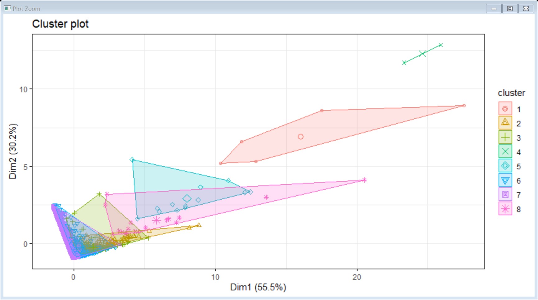
# Visualize
p3 <-fviz_cluster(km.res, kRFM_scale,
                           #plette = c("#2E9FDF", "#00AFBB", "#E7B800"), 
                           geom = "point",
                           #ellipse.type = "convex", 
                           ggtheme = theme_bw()
             )
p3

Rules v.s Clustering

# see the overlap of kmeans and handmade rules:
p5 <- ggplot(df_RFM,aes(segmentRFM,fill = kMeans_cluster))+
  geom_bar(position="stack") +
 theme(axis.text.x = element_text(angle = 90, vjust = 0.5, hjust=1))

p5

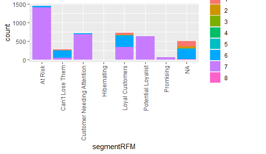
The types that are more concerned in artificial rules, Cant Lose Them, Champion and Loyal Customers and Kmeans results of clusters 6, 3, and 2 are relatively coincident, and the coincidence degree of 4 is also high, and it is located in the chanmpion category. It can be seen from the clustering results, Monetary and rencency of categories 6, 3, 2, and 4 have relatively good performance, at least none of them have obvious problem.
At risk, potential loyalist and promise are users obtained from manual rules who need greater operational efforts to recover or win, and belong to the seventh cluster in the kmeans results. The frequency, recency and monetary of this cluster are relatively middle.
Kmeans and manual rules also give different tips: in the category of loyal customers, kmeans points out that there are many users who belong to the seventh cluster. I think this part of users can be further analyzed to see if manual rules are in the classification. There are loose parts of the class.
Regardless of kmeans and manual rules, the number of categories given is relatively large, kmeans itself is more sensitive to outliers, but in our case, outliers cannot be blindly deleted. The number of users in the promising and hibernating categories is very small, and it is necessary to consider whether this category is worth operating alone, which needs to be determined in combination with the life cycle of the product.