A/B Test(2): From Start to Finish
Introduction
Several Google data scientists develops the course of A/B test in Udacity, after finishing the course there’s a final project to test the understanding of A/B test. This is the description of how I complete the final project, with an exploration on how to calculate sample size.
The Project
Background
Referring to the original description:
“ At the time of this experiment, Udacity courses currently have two options on the home page:“start free trial”, and “access course materials”. If the student clicks “start free trial”, they will be asked to enter their credit card information, and then they will be enrolled in a free trial for the paid version of the course. After 14 days, they will automatically be charged unless they cancel first. If the student clicks “access course materials”, they will be able to view the videos and take the quizzes for free, but they will not receive coaching support or a verified certificate, and they will not submit their final project for feedback.
In the experiment, Udacity tested a change where if the student clicked “start free trial”, they were asked how much time they had available to devote to the course. If the student indicated 5 or more hours per week, they would be taken through the checkout process as usual. If they indicated fewer than 5 hours per week, a message would appear indicating that Udacity courses usually require a greater time commitment for successful completion, and suggesting that the student might like to access the course materials for free. At this point, the student would have the option to continue enrolling in the free trial, or access the course materials for free instead. This screenshot shows what the experiment looks like.
The hypothesis was that this might set clearer expectations for students upfront, thus reducing the number of frustrated students who left the free trial because they didn’t have enough time—without significantly reducing the number of students to continue past the free trial and eventually complete the course. If this hypothesis held true, Udacity could improve the overall student experience and improve coaches’ capacity to support students who are likely to complete the course.
The unit of diversion is a cookie, although if the student enrolls in the free trial, they are tracked by userid from that point forward. The same userid cannot enroll in the free trial twice. For users that do not enroll, their userid is not tracked in the experiment, even if they were signed in when they visited the course overview page.”
Choosing Invariant Metrics
Invariant metrics are those shouldn’t vary between control and experiment group. It is like the alerting metrics that tells you whether the test works or not. The invariant metrics are used in sanity checks.
There are several options offered:
- Number of Cookies: That is, number of unique cookies to view the course overview page. This can be an invariant since we are allocating users based on it.
- Number of user-ids: That is, number of users who enroll in the free trial. It cannot be an invariant since the willingness to enroll is impacted by the new design.
- Click-through-probability: That is, number of unique cookies to click the “Start free trial” button divided by number of unique cookies to view the course overview page. It can be an invariant since the design only impact after clicking the ‘Start free trial’ button.
- Gross conversion: That is, number of userids to complete checkout and enroll in the free trial divided by number of unique cookies to click the “Start free trial” button. As said, enroll is impacted by the design, so it shouldn’t be the invariant.
- Retention: That is, number of userids to remain enrolled past the 14day boundary (and thus make at least one payment) divided by number of userids to complete checkout. Again, this is rather what we want to measure rather than control factors.
- Net conversion: That is, number of userids to remain enrolled past the 14day boundary (and thus make at least one payment) divided by the number of unique cookies to click the “Start free trial” button. The same as Retention.
Choosing Evaluation Metrics
The options are same as above. We wanna track the impact of the new design, so Retention and Net Conversion are selected. Gross conversion can also be measured if needed.
Measuring Variability
Before we move on to use these evaluation metrics. We want to justify our choice that these metrics are sensitive and robust. Sensitive means the metric can really detect the changes when it exists, and robust means the metric should not change from time to time out of the experiment control issues. Typically we should be really careful when the metric is complex, like nth quantile, median, etc. For those cases, we can not assume a probability distribution of the metric, so we can use A/A test to generate empirical analysis.
We are given historical data to calculate standard deviation(or standard error if consider historical data as a sample). The formula of standard error for probability, or binomial distribution is $$\sqrt{\frac{p(1-p)}{N}}$$
# historical data
pv = 40000
n_click = 3200
n_enrol = 660
p_pay_enrol = 0.53
test_size = 5000

# calculation
p_enrol_click = n_enrol/n_click
p_pay_click = p_pay_enrol * p_enrol_click # assume the two events are independent

sd_retention = math.sqrt((p_pay_enrol * (1 - p_pay_enrol)) / (test_size * (n_enrol / pv)))
sd_net_conversion = math.sqrt((p_pay_click * (1 - p_pay_click)) / (test_size * (n_click / pv)))
sd_retention
sd_net_conversion

Out[1]:0.05494901217850908
Out[2]:0.015601544582488459
The values are relatively small suggesting in natural environment they are robust. But to understand further about sensitivity and robust, we can look at historically how the two metrics change; we can also run experiment under different settings which are influential to these metrics to see how they vary(sensitivity), and run experiments in similar settings to see how they remain unchanged(robust)
Determine Sample size
The factors influence sample size are:
a)Significance level, the alpha (how much false positive rate we can tolerate);
b)Power, the beta (how much type II error we can tolerate);
In a given sample size, we must trade alpha with beta, that is, decreasing alpha is with the consequence of increasing beta and vice versa. The only we way decreases the two is by collecting more samples.
c)Baseline conversion rate for the ratios/probabilities tests. The higher the baseline conversion rate, everything equal, the large the sample we need.
d)Minimum Detectable Effect: for practical usage, what’s the minimum percentage of improvement we care? It is used to determine beta, given alpha. The smaller the minimum detectable effect, the more precise, so more samples required.
There are basically three ways to determine sample size.
-
Rule of Thumb For mean tests, there’s a general minimum sample size in statistics and applied to many companies. The formula is:
Known standard deviaion: $$ n = \frac{16\sigma^2}{\delta^2}$$. $\sigma$ is the standard deviation of evaluation metric, $\delta $ is minimum acceptable sampling error.
Unknown standard deviation: $$ n = \frac{Z^2\sigma^2}{\delta^2}$$. $Z$ is the Z-score corresponding to certain significance level. -
Statistis based Calculation
There are many research in this field, and I found 2 that is for 2 sample tests of proportion:
- Wang, H. and Chow, S.-C. 2007. Sample Size Calculation for Comparing Proportions. Wiley Encyclopedia of Clinical Trials.http://citeseerx.ist.psu.edu/viewdoc/download?doi=10.1.1.571.2708&rep=rep1&type=pdf $$n = \frac{(Z_{\alpha/2} + Z_\beta)^2(p_1(1-p_1)+p_2(1-p_2))}{(p_1-p_2)^2}$$
- R and G*Power Formula https://jeffshow.com/caculate-abtest-required-sample-size.html, also in Applied Statistics and Probability for Engineers, 3rd. Douglas C. Montgomery, George C. Runger, p. 364 $$n = \frac{[{Z_{\alpha/2}\sqrt{2\frac{(p_1+p_2)}{2}(1-\frac{(p_1+p_2)}{2})}+Z_\beta\sqrt{p_1(1-p_1)+p_2(1-p_2)}}]^2}{(p_1-p_2)^2}$$ The two above give almost identical results, see plot below.
- Python package of statsmodels.stats.proportion
Gives small numbers, see plot below.
I compared these 3 methods:
def get_size(alpha, beta, baseline, min_effect):
    '''
    alpha: significance level
    beta: statistical power = 1 - beta
    baseline: baseline conversion rate, in [0,1]
    min_effect: minimum detectable effect, in [0,1]
    return: 3 methods of sample size calculation
    '''
    import scipy.stats as st
    z_alpha = st.norm.ppf(1 - alpha / 2)
    z_beta = st.norm.ppf(1 - beta)
    p1 = baseline
    p2 = baseline + min_effect

    from statsmodels.stats.power import zt_ind_solve_power
    from statsmodels.stats.proportion import proportion_effectsize as es

    size = ((z_alpha + z_beta) ** 2 * (p1 * (1 - p1) + p2 * (1 - p2))) / (p1 - p2) ** 2
    size2 = (z_alpha * math.sqrt((p1 + p2) * (1 - p1 + 1 - p2) * 0.5) + z_beta * math.sqrt(p1 * (1 - p1) + p2 * (1 - p2))) ** 2 / (p1 - p2) ** 2
    size3 = zt_ind_solve_power(effect_size=es(prop1=p1, prop2=p2), alpha=alpha, power=beta, alternative="two-sided")

    return size, size2, size3

nums = np.linspace(0.01,0.95,100)
size_1, size_2, size_3= [],[],[]
for i in nums:
    num1, num2, num3 = get_size(alpha = 0.05, beta = 0.2, baseline = i, min_effect = 0.01 if (i>0.001 and i+0.01 < 1) else 0)
    size_1.append(num1)
    size_2.append(num2)
    size_3.append(num3)

lines = pd.DataFrame({
    'probability':nums,
    'size_1':size_1,
    'size_2':size_2,
    'size_3':size_3
})

import seaborn as sns
sns.lineplot(x='probability', y='value', hue='variable',
             data=pd.melt(lines, ['probability']), alpha = 0.3)
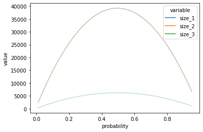
1 and 2 overlapps for most of time, and the package generates very small result. Both sample sizes reaches maximum when baseline effect getting close to 50%.
- Using standard error to calculate Another method is to calculate by the relationship between alpha and beta, it’s possibly not restricted to 2 sample proportion test.
from scipy.stats import norm
# Inputs:
#   The desired alpha for a two-tailed test
# Returns: The z-critical value
def get_z_star(alpha):
    return norm.ppf((1-alpha/2))

# Inputs:
#   z-star: The z-critical value
#   s: The standard error of the metric at N=1
#   d_min: The practical significance level
#   N: The sample size of each group of the experiment
# Returns: The beta value of the two-tailed test
def get_beta(z_star,s, d_min, N):
    SE = s /  math.sqrt(N)
    return norm.cdf(z_star*SE,d_min,SE)

# Inputs:
#   s: The standard error of the metric with N=1 in each group
#   d_min: The practical significance level
#   Ns: The sample sizes to try
#   alpha: The desired alpha level of the test
#   beta: The desired beta level of the test
# Returns: The smallest N out of the given Ns that will achieve the desired
#          beta. There should be at least N samples in each group of the experiment.
#          If none of the given Ns will work, returns -1. N is the number of
#          samples in each group.
def required_size(s, d_min, Ns=200000, alpha=0.05, beta=0.2):
    z=get_z_star(alpha)
    for N in range(1,Ns):
        if get_beta(z, s, d_min, N) <= beta:
            return N
    return -1

## Plot: vary N and see how beta changes, every thing equal
s = math.sqrt(p_pay_enrol*(1-p_pay_enrol)/n)
N = range(1, 20000)
beta = []
z_star = 1.96
for n in N:
    SE = s /  math.sqrt(n)
    beta.append(norm.cdf(z_star*SE,d_min,SE))

betas = pd.DataFrame({
    'N':N,
    'beta':beta
})

sns.lineplot(x='N', y='beta',
             data=betas, alpha = 0.3)
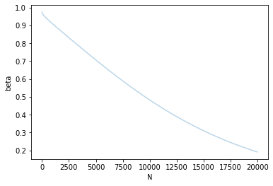
So as sample size N increases, the type II error of not rejecting false hypothesis decreases as expected.
Finally I use statistics method and standard error methods to get the sample size:
## Statistic methods
base_retention = p_enrol_click
base_conversion = p_pay_enrol
retention = get_size(alpha=0.05, beta=0.2, baseline=base_retention, min_effect=0.01)
conversion = get_size(alpha=0.05, beta=0.2, baseline=base_conversion, min_effect=0.01)
# since we cannot control the number of click and enrol, we need to use historical data to get total pvs for click and control.
inv_p_click =  pv/ n_click
inv_p_enrol =  pv / n_enrol
re_lst = [float(x) * 2 * inv_p_click for x in retention]
conv_lst = [float(x) * 2 * inv_p_enrol for x in conversion]
math.ceil(max(max(re_lst), max(conv_lst)))

Out[3]:4733446

## Standard Error method
"""number of clickes needed for net_conversion"""
click_through_probability=0.08
n=1 ## Start the guessing from 1
s=math.sqrt(p_pay_click*(1-p_pay_click)/n)
d_min=0.0075
req=required_size(s,d_min)
print("number of clicks needed for net_conversion:",int(req))
print("number of pageviews needed for net_conversion:",int(req/click_through_probability))

Out[4]:'number of clickes needed for net_conversion'
		'number of clicks needed for net_conversion: 13586'
		'number of pageviews needed for net_conversion: 169825'

"""number of enrollment needed for retention"""
n=1
s=math.sqrt(p_pay_enrol*(1-p_pay_enrol)/n)
d_min=0.01
req=required_size(s,d_min)
print("number of clicks needed for retention:",int(req))
print("number of pageviews needed for retentionn:",int(req/(n_enrol/pv)))

Out[5]:'number of enrollment needed for retention'
		'number of clicks needed for retention: 19552'
		'number of pageviews needed for retentionn: 1184969'
Sanity Check
In this example we collect data for 30 days, note down every metric of each day.
Assume we now complete the data collection, we first need to perform sanity check as mentioned before.
The way we do sanity check is to calculate confidence interval for the invariant. If our measured statistics falls in theoratical confidence interval, it passes the sanity check. The formula for 2 mean test margin of error is:
$$margin \space of \space error = Z_\alpha \sqrt{\frac{p(1-p)}{N_{total}}}$$
Confidence interval is $$[point \space estimate - margin \space of \space error, point \space estimate + margin \space of \space error]$$
For 2 sample proportional test, the formula is:
$$margin \space of \space error = \sqrt{P_{pool}(1-P_{pool})(\frac{1}{N_{control}}+\frac{1}{N_{experiment}})}$$
where $$P_{pool} = \frac{N_{control=1}+N_{experiment=1}}{N_{control}+N_{experiment}}$$
def get_CI_mean(alpha, control_cnt, expr_cnt, p):
    '''
    alpha: significance level
    control_cnt: control group size
    expr_cnt: experiment group size
    p: point estimate
    '''
    sd = math.sqrt(0.5 * 0.5 / (control_cnt + expr_cnt))
    import scipy.stats as st
    z_alpha = st.norm.ppf(1 - alpha / 2)
    margin_error = sd * z_alpha
    return(p - margin_error, p + margin_error)

print(sum(pageviews_exp)/(sum(pageviews_cont)+sum(pageviews_exp)), get_CI_mean(0.05, sum(pageviews_cont), sum(pageviews_exp), 0.5))
print(sum(clicks_exp)/(sum(clicks_cont)+sum(clicks_exp)), get_CI_mean(0.05, sum(clicks_cont), sum(clicks_exp), 0.5))

Out[6]:0.4993603331193866 (0.4988204138245942, 0.5011795861754058)
	   0.49953265259333723 (0.4958845713471463, 0.5041154286528536)

def get_CI_prop(alpha, control_true, exp_true, control_sum, exp_sum, phat):

    prob_pool =  (control_true + exp_true) / (control_sum + exp_sum)
    se = math.sqrt(prob_pool * (1 - prob_pool) * (1 / control_sum + 1 / exp_sum))
    import scipy.stats as st
    z_alpha = st.norm.ppf(1 - alpha / 2)

    margin_error = se * z_alpha
    return( phat - margin_error, phat + margin_error)

get_CI_prop(0.05, sum(clicks_cont), sum(clicks_exp), sum(pageviews_cont), sum(pageviews_exp), 0)

Out[7]: (-0.001295655390242568, 0.001295655390242568)
So as all point estimate falls in the confidence interval, the sanity check is passed.
Effect Size Test
Now we measure the experiment metrics. The logic is the same: if point estimate falls in the confidence interval, then the 2 groups does not differ significantly at the alpha level.
### retention: enroll --> payment
n = len(payment_exp)
sum_payment_cont=sum(payment_cont[:n])
sum_payment_exp=sum(payment_exp[:n])
sum_enroll_cont=sum(enrolls_cont[:n])
sum_enroll_exp=sum(enrolls_exp[:n])
p_hat = sum_payment_exp / sum_enroll_exp - sum_payment_cont / sum_enroll_cont
p_hat
get_CI_prop(0.05, sum_payment_cont, sum_payment_exp, sum_enroll_cont, sum_enroll_exp, p_hat)

Out[8]:0.031094804707142765
(0.008104858181445022, 0.05408475123284051)

### net conversion: clicks --> payment
n=len(enrolls_exp)
sum_clicks_cont=sum(clicks_cont[:n])
sum_clicks_exp=sum(clicks_exp[:n])
sum_payment_cont=sum(payment_cont[:n])
sum_payment_exp=sum(payment_exp[:n])
p_hat = sum_payment_exp/sum_clicks_exp-sum_payment_cont/sum_clicks_cont
p_hat
get_CI_prop(0.05, sum_payment_cont, sum_payment_exp, sum_clicks_cont, sum_clicks_exp, p_hat)

Out[9]:-0.0048737226745441675
(-0.011604500677993734, 0.0018570553289053993)
So both metrics falls in the confidence interval, there’s no significant different in retention and conversion in the experiment group and control group.
Sign Test
To further verify the result, we perform sign test to see in less power, if the test is significant.
(We can further see if it’s in weekend or week days that differ much, but I am too lazy to do that.)
from scipy.stats import wilcoxon
n = len(payment_exp)
retention_exp = [x/y for x,y in zip(payment_exp[:n], enrolls_exp[:n])]
retention_cont = [x/y for x,y in zip(payment_cont[:n], enrolls_cont[:n])]

wilcoxon(retention_exp, retention_cont)

Out[10]:WilcoxonResult(statistic=107.0, pvalue=0.36039113998413086)

n=len(enrolls_exp)
conversion_exp = [x/y for x,y in zip(payment_exp[:n], clicks_exp[:n])]
conversion_cont = [x/y for x,y in zip(payment_cont[:n], clicks_cont[:n])]

wilcoxon(conversion_exp, conversion_cont)

Out[11]:WilcoxonResult(statistic=120.0, pvalue=0.6010458469390869)
So the sign test also suggest our metrics do not differ.
Conclusion
We selected proper metrics to guarantee the effectiveness of our experiment. But finally the result suggests at a significant level, and error level we care, we should not launch the experiment.